
- How to use different display modes for 1D arrayed spectra
- How to navigate throughout the different subspectra in the arrayed item
- How to process individual spectra separately
When an arrayed experiment has been detected, all subspectra are grouped together and plotted in the stacked display mode in Mnova (see figure below). Several points are worth mentioning:
(A). Take a look at the green box in the figure below: it shows the so-called ‘active spectrum’. What does this mean?
The concept of active spectrum is easier to illustrate with the following example: as I wrote in my previous post, in general all the spectra in an arrayed item are processed exactly with the same processing operations. For example, same level of zero filling, same apodization function, same FT type, same phase correction, etc. However, it i’s possible that some particular spectra require a slightly different processing, independently from the others. In order to do that, it i’s necessary to deactivate the ‘Apply Processing to All spectra in Stack’ option.
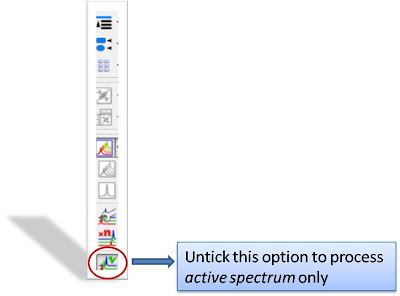
So if that option is off, any processing operation will be applied only to the active spectrum in the stack.
The question is: how can we change the active spectrum? There are 3 different ways:
- Just click on the spectrum you want to be active. This is probably the most intuitive way.
- Use SHIFT + Mouse Wheel to navigate throughout all the spectra in the stack, one after the other.
- Use SHIFT + Up/Down arrow keys. This is analogous to point 2)
(B). If the number of subspectra (traces) is large (e.g. > 10), working in the stack mode might not be very practical. Quite often, working only with the active spectrum on the screen will be a much better option. This mode can be activated as shown in the image below.
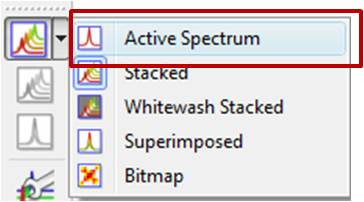

While working on this mode, you will see on the screen just the active spectrum. Should you want to move to another spectrum without resorting to the stack mode, just use methods 2) and 3) described above (Shift+Mouse Wheel or Shift + Up/Down keys).
IMPORTANT: Remember that even if only the active spectrum is visible, unless the “Apply Processing to All spectra in Stack” option is off, all spectra in the stack will also be processed.(C) Another useful display mode consists of superimposing all subspectra (see figure below). This method is very useful, for example, when you want to check whether some peaks shift their position (for instance, due to differences in pH, temperature, etc., as is common in biofluids spectra).

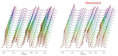
Finally, there is an additional display mode, the so called whitewashed stacked plot. The whitewashing effect means that the spectra at the front of the display hide the spectra behind them from view, as depicted in the figure below.
In my next post I will show how to extract useful information from arrayed spectra.

This plotting mode can be useful to create nice reports, but it’s important to emphasize that drawing time will be significantly higher than with the other plotting modes, so it is not recommended when processing the spectra in real time (e.g. interactive phase correction).
In my next post I will show how to extract useful information from arrayed spectra.
No comments:
Post a Comment